Lecture Notes - ramblingeconomist.in

Please feel free to use this for your classes. Just acknowledge my name. Thanks!

Auctions:

I am going to concentrate on one topic rather than doing a survey of the extensive literature that exists for this topic. You can see that many types of auctions exist, look here:

http://en.wikipedia.org/wiki/Auction

There are many topics here that are of interest for both serious theoretical and empirical research:

What are the optimal bidding strategies for each type of auction? How does it depend on the information that the bidders have about a. the value of the item, b. the value that other sellers place on the item and c. the real-time bidding process of the auction?

How do prices in the auction market deviate (or not) from competitive prices or oligopoly prices?

What is the role of signaling in auction markets? How do bids convey information to other potential buyers?

We will look at only one problem:

Assume only one object is being auctioned. The format is sealed-bid first price auction, the winner gets the object and pays his bid “b”. If the value of the object to him is v, he gains v-b if he wins, and zero if he does not win.

If there are two bidders, and they value the same object v₁ and v₂ respectively, and if there is perfect information, and v₁ > v₂, bidder 1 would bid v₂+ e, when e is a very small number and bidder 2 will bid v₂. Of course 1 would win and have a gain of v₁ – v₂ .

The problem becomes interesting if we assume that there are two bidders, but they do not know each other’s valuations. Without losing generality, we assume that t_i is valuation of type i, and t_iis known to be uniformly distributed over [0,1].

In a Bayesian Nash equilibrium, what would be the equilibrium bidding strategy of t_i ? This is the question we answer:

If t_i wins by bidding b, he gets t_i – b if his bid is higher than the other bid, otherwise he gets zero.

Therefore, t_i’s expected profit from bidding an amount b is

Π_i = (t-b) prob(b_j < b)

We manipulate the term prob(b_j < b) a little bit. Assume that a player with valuation t will have an equilibrium bid b*(t). Since the game is symmetric, both players will use the same bidding strategy in equilibrium. Further, the function b*(t) is monotonically increasing, which means higher t will induce a higher bid in equilibrium.

Therefore prob(b_j < b) = prob(b*(t_j) < b) = prob( t_j < ϕ(b)) when ϕ(b) = inverse of b*(t).

But then prob( t_j < ϕ(b)) = ∫^ϕ(b) xdx = ϕ(b), because of our assumption of uniform distribution of valuations.

So, in equilibrium, player “i” with valuation t_i will maximize

Π_i = (t_i-b) prob(b_j < b) = (t-b) ϕ(b), by choosing his bid b

Therefore the first order-condition, described below will be met for every t

∂ Π_i /∂b = 0 = – ϕ(b) + (t-b) dϕ/db = 0

So, every t will bid according to above and in equilibrium every t will follow his equilibrium bidding strategy which implies that b= b*(t) or t = ϕ(b*)

Therefore, for any b* we will have

– ϕ(b*) + (ϕ(b*) –b*) dϕ(b*)/db = 0

Since every b* will satisfy the above, we may think of this as a simple differential equation in b

A note on differential equations:

Solution of a differential equation:

-y + (y-x)dy/dx = 0

Rewrite as

-ydx –xdy + y dy = 0

(ydx + xdy) = ydy

Define a change of variables

Let z = xy, then dz = xdy + ydx

So we have, dz = ydy or taking integrals on both sides

z = y²/2 or xy = y²/2 or y = 2x (done)

Finally we apply this to get ϕ(b*) = 2b or b = ϕ(b*)/2

Or b*(t) = t/2

So every player, regardless of his own valuation, will bid half of his valuation in this game.

So, for example, expected profit of someone with valuation 75c will be

Profit = (3/4 – 3/8) prob(t < 3/8) = (3/8) (3/8)

Market for network services

Although the first paper on network issues was written by Rohlfs in 1974, network goods (or services) have become a very important part of most advanced economies .

What follows is my first lecture on “Network Services”, used frequently in Industrial Organization Courses

What is the difference between an ordinary service, say a haircut and a network service, for instance telephone service?

Haircut (only I look ugly as before!!)

The consumer who is getting a haircut gains utility from it, hopefully, and no one else is affected. But the utility one gets from having a phone depends on how many other people have telephones. So one consumer’s utility depends on the total number of buyers of the service.

Networking!!

We will discuss two market structures, monopoly and duopoly in the network market, also compare this with the social optimum solution. As we will see, the nature of equilibrium is substantially different from non-network goods.

First we derive the demand curve of a network service. Unlike non-network goods and services, the demand curve is not negatively sloped! This changes the nature of equilibrium.

Assume that consumers pay a single price p for accessing the network , but there is no charge for subsequent pay per use.

N is potentially the maximum number of consumers that may want to subscribe to the network.

Let v_i be the value that consumer “i” places on the network when everyone subscribes to the network. In other words, v_i is the maximum amount that “i” will pay for the network.

If all consumers are identical, then this is an easy model to analyze, but that is not a realistic assumption. So we assume that customers are different. They are distributed uniformly over the interval [0,100].

So, if the consumer knows that f is the fraction of total consumers subscribing to the network, the maximum that consumer “i” would pay is a function of f and v_i. For simplicity, we assume that the consumer “i” will pay f.v_i.

Therefore given a price p, there will be a consumer whose willingness to pay is v_i^ such that

The price p = f v_i^.

By our assumption of uniform distribution, the fraction of consumers who want to subscribe to this service is 1 – f = v_i^/100

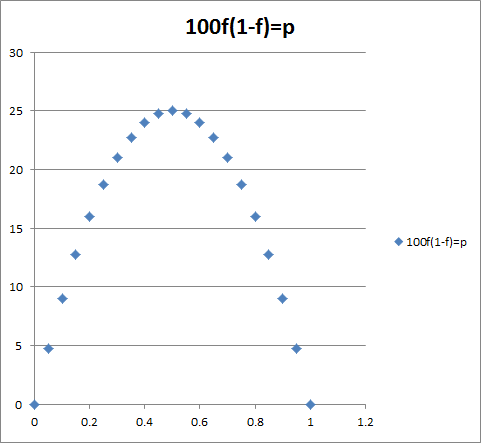
Therefore p = 100f(1-f) after a little algebra

This is the demand curve for network services, note that this is inverse demand showing p as a function of f, when f is the fraction of the total subscribing to the network.

“f” is fraction of people in the network	p is demand price
0	0
0.1	9
0.2	16
0.3	21
0.4	24
0.5	25
0.6	24
0.7	21
0.8	16

This demand curve is not negatively sloped.

It is positively sloped for f < ½ , reaching a maximum at p = 25.

Over the positively sloped range, some consumers quit (f falls), there are two effects:

Due to the price effect, demand price goes up (the people who would want to pay higher price would remain in the market)

Due to the network effect, the value of the network falls to existing customers, so some others quit as well.

As the network effect dominates the price effect over this range, as f falls, demand price p also falls

Over the negatively sloped range, the network effect is small because f is large, and the demand curve is negatively sloped.

Assuming Q = fN, we get the total revenue curve as

Q = pfN = 100f(1-f)fN = 100f²N – 100f³N

Network monopoly with marginal cost of 11.11 (no fixed costs)

My numbers are a little different from the ones in text , pages 642-3.

Π = pfN – (11.11)fN

= 100f(1-f).fN -11.11fN

Differentiating with respect to f, and setting to zero

100f(2-3f)N-11.11N = 0

2f – 3f² – 11.11/100 = 0

Or 3f²-2f + (1/9) = 0

The solution is

Optimal f* = 1/6 {2 ±( 4 – 4x2x(1/9)}^1/2

Which comes to f* = 0.6, p* = 24, and profit per-unit as 13.49

Total profit is 13.49N

We try zero marginal cost next

Π = pfN

= 100f(1-f).fN

Check the solution is f = 2/3, p = 100(2/3)(1/3) = 22.22

Profit per-unit is 22.22 (2/3) N = 14.8N

If price is zero, then everyone subscribes, total demand is N

The total social surplus is 1/6 N

The government may supply this for free and charge a tax per user of 1/6 ?

The other problem is how a network is built over time. In regular market as a price is announced, there could be a fraction of the total number of buyers at first, but the rest would come over time.

In a network market, a fraction of buyers may come initially, but if f is less than the breakeven point, the network may collapse if some decide to leave.

Network duopoly with Marginal cost 11.11

There is a Bertrand solution with price = 11.11.

But there is also another Nash equilibrium where one sells at the monopoly price and the other sells at 11.11 with zero customers. Because of the network externality, the firm with price 11.11 will not get any customers, if the monopoly is there first.

Interestingly, entry is also not possible here if there is a monopoly. One way to enter would be a dynamic strategy where the entrant offers it at a zero price, at a loss. Then the incumbent will either offer a zero price or exit. If the incumbent offers a zero price, they can both increase their price to 11.11 and make normal profits.

Alternately, because of network externality, any initial provider should provide the service at well below cost or for free and charge a one-time sign up fee. This would establish a large network, and new entry would be blocked since cost per period for the consumers is zero.

Lastly we generalize the monopoly model with and without fixed cost with the assumption that the consumers’ willingness to pay is uniformly distributed on an interval [0,K]. Here

P = Kf(1-f) and

Π = pfN

= Kf(1-f).fN

Here, the monopoly price would be a function of K

Notice that the breakeven price is P = K/2

Category: Lecture Notes

Auctions: Lecture Notes

Lecture Notes – Market for Network Services